The optimization problem

\[\begin{split} \begin{array}{lll} \textrm{minimize} & f(x) & \\ \textrm{subject to} & g_{i}(x) \leq 0, & i = 1, \ldots, m, \\ & h_{j}(x) = 0, & j = 1, \ldots, p, \\ \end{array} \end{split}\]

• \(x = (x_{1}, x_{2}, \ldots)\): optimization variables

• \(f \colon \mathcal{X} \to \mathbb{R}\): objective function

• \(g_{i} \colon \mathcal{X} \to \mathbb{R}, i = 1, \ldots, m\): inequality constraint functions

• \(h_{j} \colon \mathcal{X} \to \mathbb{R}, j = 1, \ldots, p\): equality constraint functions

Decision set \(\mathcal{X}\) may be finite \(\mathbb{R}^{n}\), a set of matrices, a discrete set \(\mathbb{Z}^{n}\), or an infinite dimensional set.

Constraint functions \(g_{i}(x)\) and \(h_{j}(x)\) limit the decision set \(\mathcal{X}\) to a set of feasible points \(x \in X \subset \mathcal{X}\).

The Optimal solution \(x^{*} \in X\) has smallest value of \(f\) among all feasible points that “satisfy the constraints”:

\[ \forall x \in X \colon f(x^{*}) \leq f(x). \]

Classes of optimizations problems

• Unconstrained optimization: \(m = p = 0\)

• Constrained optimization \(m > 0\) or \(p > 0\)

• Linear Programming: \(f\) linear, \(g_{i}\), \(h_{j}\) affin-linear

• Quadratic Programming: \(f(x) = \frac{1}{2}x^{T}Ax + b^{T}x +c\), \(g_{i}\), \(h_{j}\) affin-linear

• Convex Optimization: \(f\) convex, \(g_{i}\) convex, \(h_{j}\) affin-linear

Local and global optima

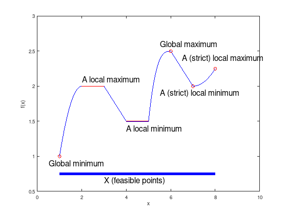
Consider the following piece-wise defined function:

f = {@(x) -(x - 2).^2 + 2, ...
     @(x) 2, ...
     @(x) -(x - 7) / 2, ...
     @(x) 3/2, ...
     @(x) (x - 6).^3 + 5/2, ...
     @(x) -(x - 11) / 2, ...
     @(x) (x - 7).^2 / 4 + 2};
for i = 1:7
  fun = f{i};
  x = linspace (i, i + 1, 40);
  y = fun (x);
  plot (x, y, 'b');
  hold on;
end
xlim ([0, 10]);
ylim ([0.5, 3]);
xlabel ('x');
ylabel ('f(x)');
fmt = {'FontSize', 16};
plot (1, 1.00, 'ro'); text (0.5, 0.9, 'Global minimum', fmt{:});
plot (6, 2.50, 'ro'); text (5.5, 2.6, 'Global maximum', fmt{:});
plot (7, 2.00, 'ro'); text (5.5, 1.9, 'A (strict) local minimum', fmt{:});
plot (8, 2.25, 'ro'); text (6.5, 2.4, 'A (strict) local maximum', fmt{:});
plot (2:3, [2, 2],     'r'); text (2, 2.1, 'A local maximum', fmt{:});
plot (4:5, [3, 3] / 2, 'r'); text (4, 1.4, 'A local minimum', fmt{:});
plot ([1, 8], [0.75, 0.75], 'b', 'LineWidth', 6);
text (3, 0.65, 'X (feasible points)', fmt{:});

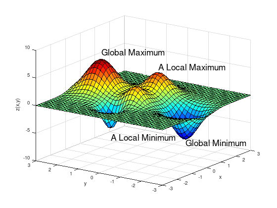
Local and global optima of a two-dimensional function.

N = 3;
[X,Y] = meshgrid (linspace (-N, N, 40));

% Gaussian probability density function (PDF)
GAUSS = @(sigma, mu)  1 / (sigma * sqrt (2*pi)) * ...
                      exp (-0.5 * ((X - mu(1)).^2 + (Y - mu (2)).^2) / sigma^2);

Z = 9 * GAUSS (0.6, [ 0.0,  2.0]) + 5 * GAUSS (0.5, [ 1.0,  0.0]) ...
  + 3 * GAUSS (0.4, [-0.5,  0.0]) - 3 * GAUSS (0.3, [-1.5,  0.5]) ...
  - 7 * GAUSS (0.5, [ 0.0, -2.0]);

surf (X, Y, Z);
xlabel ('x');
ylabel ('y');
zlabel ('z(x,y)');
colormap ('jet');
props = {'FontSize', 18};
text ( 0.0, -2.0, -6.2, 'Global Minimum', props{:});
text ( 0.0,  2.0,  7.2, 'Global Maximum', props{:});
text (-1.5,  0.5, -5.5, 'A Local Minimum', props{:});
text ( 1.0,  0.0,  5.0, 'A Local Maximum', props{:});
view (-55, 21)

Two-dimensional constrained example

A simple problem can be defined by the constraints

\[\begin{split} \begin{array}{l} x_1 \geq 0, \\ x_2 \geq 0, \\ x_1^2 + x_2^2 \geq 1, \\ x_1^2 + x_2^2 \leq 2, \end{array} \end{split}\]

with an objective function to be maximized

\[ f(x) = x_1 + x_2 \]

subplot (1, 2, 1);

% Visualize constrained set of feasible solutions (blue).
circ = @(x) sqrt (max(x)^2 - x.^2);
x_11 = 0:0.01:sqrt(2);
x_21 = circ (x_11);
x_12 = 1:-0.01:0;
x_22 = circ (x_12);
area ([x_11, x_12], [x_21, x_22], 'FaceColor', 'blue');

% Visualize level set of the objective function (magenta)
% and its scaled gradient (red arrow).
hold on;
plot ([0 2], [2 0], 'LineWidth', 4, 'm');
quiver (1, 1, 0.3, 0.3, 'LineWidth', 4, 'r');
axis equal;
xlim ([0 2]);
ylim ([0 2]);
xlabel ('x_1');
ylabel ('x_2');
title ('Contour plot');

subplot (1, 2, 2);
[X1, X2] = meshgrid (linspace (0, 1.5, 500));
FX = X1 + X2;

% Remove infeasible points.
FX((X1.^2 + X2.^2) < 1) = inf;
FX((X1.^2 + X2.^2) > 2) = inf;
surf (X1, X2, FX);
shading flat;
colormap ('jet');
hold on;
plot3 (1, 1, 2, 'ro');
axis equal;
xlabel ('x_1');
ylabel ('x_2');
zlabel ('f(x)');
title ('3D plot');
view (11, 12);

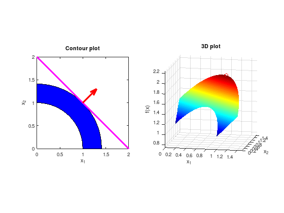
The intersection of the level-set of the objective function (\(f(x) = 2 = const.\)) and the constrained set of feasible solutions represents the solution.

\(\max f(x) = -\min -f(x)\)

In these lectures we are mainly interested in methods for computing local minima.

Notation

Vectors \(x \in \mathbb{R}^{n}\) are column vectors. \(x^{T}\) is the transposed row vector.

A norm in \(\mathbb{R}^{n}\) is denoted by \(\lVert \cdot \rVert\) and corresponds to the Euclidean norm:

\[ \lVert x \rVert = \lVert x \rVert_{2} = \left( x^{T}x \right)^{\frac{1}{2}} = \sqrt{x_{1}^{2} + \ldots + x_{n}^{2}}. \]

Is \(\lVert \cdot \rVert\) a norm on \(\mathbb{R}^{n}\), then

\[ \lVert A \rVert := \max\left\{ \lVert Ax \rVert \colon \lVert x \rVert \leq 1 \right\} \]

defines the matrix norm (operator norm) for \(A \in \mathbb{R}^{n \times n}\).

For the Euclidean vector norm this is

\[ \lVert A \rVert = \sqrt{\lambda_{\max}(A^{T}A)} = \sigma_{\max}(A), \]

where \(\lambda_{\max}(\cdot)\) denotes the maximal eigenvalue and \(\sigma_{\max}(\cdot)\) the maximal singular value of a matrix.

The open ball with center \(x \in \mathbb{R}^{n}\) and radius \(\varepsilon > 0\) is denoted by

\[ B_{\varepsilon}(x) := \{ y \in \mathbb{R}^{n} \colon \lVert y - x \rVert < \varepsilon \} = \{ x + \varepsilon u \in \mathbb{R}^{n} \colon \lVert u \rVert \leq 1 \}. \]

The interior of a set \(X \subset \mathbb{R}^{n}\) is denoted by \(\operatorname{int}(X)\) and the border by \(\partial X\). For \(x \in \operatorname{int}(X)\) and \(\varepsilon > 0\) there is \(B_{\varepsilon}(x) \subset X\).

A subset \(X \subset \mathbb{R}^{n}\) is called “open”, if \(int(X) = X\). (“The border \(\partial X\) is not included.”)

A closed subset \(X \subset \mathbb{R}^{n}\) is called “compact”, if every open cover of \(X\) has a finite sub-cover. (“No holes in \(X\), border included.”).

In the notation \(f \colon X \to Y\), the set \(X\) is the domain of \(f\) and is alternatively denoted as \(\operatorname{dom}(f)\).

Let \(f \colon \mathbb{R}^{n} \to \mathbb{R}\) be continuously differentiable (\(f \in C^{1}(\mathbb{R}^{n},\mathbb{R})\)), then the gradient of \(f\) in \(x\) is denoted by the column vector:

\[\begin{split} \nabla f(x) = \begin{pmatrix} \dfrac{\strut\partial}{\strut\partial x_{1}} f(x) \\ \vdots \\ \dfrac{\strut\partial}{\strut\partial x_{n}} f(x) \end{pmatrix} \end{split}\]

Let \(f \colon \mathbb{R}^{n} \to \mathbb{R}\) be twice continuously differentiable (\(f \in C^{2}(\mathbb{R}^{n},\mathbb{R})\)), then the symmetric Hessian matrix of \(f\) in \(x\) is denoted by:

\[\begin{split} \nabla^{2} f(x) = \begin{pmatrix} \dfrac{\strut\partial^{2}}{\strut\partial x_{1}\strut\partial x_{1}} f(x) & \cdots & \dfrac{\strut\partial^{2}}{\strut\partial x_{1}\strut\partial x_{n}} f(x) \\ \vdots & \ddots & \vdots \\ \dfrac{\strut\partial^{2}}{\strut\partial x_{n} \strut\partial x_{1}} f(x) & \cdots & \dfrac{\strut\partial^{2}}{\strut\partial x_{n} \strut\partial x_{n}} f(x) \end{pmatrix} \end{split}\]

A real symmetric matrix \(A \in \mathbb{R}^{n \times n}\) is positive semi-definte, if \(d^{T}Ad \geq 0\) for all \(d \in \mathbb{R}^{n} \setminus \{ 0 \}\) and is denoted by \(A \succeq 0\).

A real symmetric matrix \(A \in \mathbb{R}^{n \times n}\) is positive definte, if \(d^{T}Ad > 0\) for all \(d \in \mathbb{R}^{n} \setminus \{ 0 \}\) and is denoted by \(A \succ 0\).

The Landau symbol is defined by

\[ \phi(d) = o\left(\lVert d \rVert^{k}\right) \iff \lim_{d \to 0} \frac{\phi(d)}{\lVert d \rVert^{k}} = 0. \]

Taylor’s theorem (only linear and quadratic)

Let \(f \in C^{1}(\mathbb{R}^{n},\mathbb{R})\), \(X \subset \mathbb{R}^{n}\) open, \(x \in X\), \(d \in \mathbb{R}^{n}\) and \(\lVert d \rVert\) sufficiently small, then:

\[ f(x + d) = f(x) + \nabla f(x)^{T}d + o(\lVert d \rVert). \]

Additionally, if \(f \in C^{2}(\mathbb{R}^{n},\mathbb{R})\) and for \(0 < \theta < 1\), the remainder is expressible by

\[ f(x + d) = f(x) + \nabla f(x)^{T}d + \frac{1}{2}d^{T}\nabla^{2} f(x + \theta d)d. \]

Let \(f \in C^{2}(\mathbb{R}^{n},\mathbb{R})\), \(X \subset \mathbb{R}^{n}\) open, \(x \in X\), \(d \in \mathbb{R}^{n}\) and \(\lVert d \rVert\) sufficiently small, then:

\[ f(x + d) = f(x) + \nabla f(x)^{T}d + \frac{1}{2}d^{T}\nabla^{2} f(x)d + o(\lVert d \rVert^{2}). \]

Theorem 1: Extreme value theorem

Let \(X \subset \mathbb{R}^{n}\) non-empty and compact and \(f \colon \mathbb{R}^{n} \to \mathbb{R}\) continuous. Then there exists a global minimum of \(f\) over \(X\).

If a real-valued function \(f\) is continuous on the closed interval \([a,b]\), then \(f\) must attain a maximum and a minimum, each at least once!