UM03

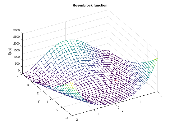
Consider the Rosenbrock function

\[ f(x,y) = (a - x)^2 + b \left( y - x^2 \right)^2. \]

It has a global minimum at \(P_{1} = (a, a^2)\) with \(f(P_{1}) = 0\). In this exercise the parameters \(a = 1\) and \(b = 100\) are chosen, as in many books on mathematical optimization.

\[\begin{split} \nabla f = \begin{pmatrix} -2(a - x) - 4bx(y - x^2) \\ 2b(y - x^2) \end{pmatrix} \end{split}\]

\[\begin{split} \nabla^{2} f = \begin{pmatrix} 2 - 4by + 12bx^2 & -4bx \\ -4bx & 2b \end{pmatrix} \end{split}\]

1. Create a plot of \(f\) for \(-2 \leq x \leq 2\) and \(-1 \leq y \leq 4\).

f = @(x,y) 100 * (y - x.^2).^2 + (1 - x).^2;
[x, y] = meshgrid (linspace (-2, 2, 30), linspace (-1, 4, 30));
mesh (x, y, f(x,y));
grid on;
xlabel ('x');
ylabel ('y');
zlabel ('f(x,y)');
title ('Rosenbrock function');
hold on;
plot3 (1, 1, 0, 'ro');
view (-30, 50);

2. Numerical experiments.

Study um03_experiment in Matlab/Octave. Repeat this exercise with other well-known Test functions for optimization.