UM02

Consider the function \(f(x,y) = x^{3} - 6xy + 8y^{3}\).

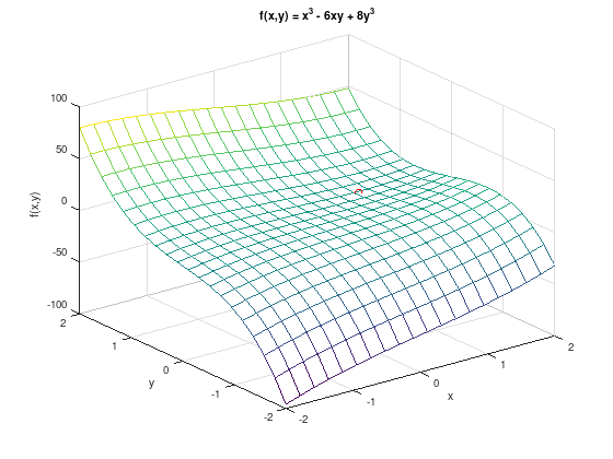
1. Create a plot of \(f\) for \(-2 \leq x,y \leq 2\).

f = @(x,y) x.^3 - 6.*x.*y + 8.*y.^3;

[x, y] = meshgrid (linspace (-2, 2, 20));
mesh (x, y, f(x,y));
grid on;
xlabel ('x');
ylabel ('y');
zlabel ('f(x,y)');
title ('f(x,y) = x^3 - 6xy + 8y^3');
hold on;
plot3 (1, 0.5, -1, 'ro');

2. Compute the gradient \(\nabla f\) and the Hessian matrix \(\nabla^{2} f\).

Solution:

\[\begin{split} \nabla f = \begin{pmatrix} 3x^{2} - 6y \\ 24y^{2} - 6x \end{pmatrix} \end{split}\]

\[\begin{split} \nabla^{2} f = \begin{pmatrix} 6x & -6 \\ -6 & 48y \end{pmatrix} \end{split}\]

3. Compute all stationary points and the respective function values.

Solution:

Stationary points: \(\nabla f = 0\).

\[\begin{split} \begin{aligned} 3x^{2} - 6y &= 0 \\ 24y^{2} - 6x &= 0 \\ \end{aligned} \end{split}\]

From the first equation follows \(y = \frac{1}{2} x^{2}\). The resulting equation

\[ 6x^{4} - 6x = 0 \iff (x^{3} - 1) x = 0 \]

yields the stationary points \(P_{1} = (0,0)^{T}\) with \(f(P_{1}) = 0\) and \(P_{2} = (1,0.5)^{T}\) with \(f(P_{2}) = -1\).

4. Classify all stationary points.

Solution:

Hessian matrix at \(P_{1}\):

\[\begin{split} \nabla^{2} f(P_{1}) = \begin{pmatrix} 0 & -6 \\ -6 & 0 \end{pmatrix} \end{split}\]

Classification with eigenvalues (roots of the characteristic polynomial):

\[\begin{split} 0 = \det\begin{pmatrix} -\lambda & -6 \\ -6 & -\lambda \end{pmatrix} = \lambda^{2} - 36 \end{split}\]

\[ \Rightarrow \lambda_{1/2} = \pm \sqrt{36} = \pm 6 \]

The roots of the characteristic polynomial are positive and negative. Thus the Hessian matrix is indefinite and \(P_{1}\) is a saddle point.

Hessian matrix at \(P_{2}\):

\[\begin{split} \nabla^{2} f(P_{2}) = \begin{pmatrix} 6 & -6 \\ -6 & 24 \end{pmatrix} \end{split}\]

Classification with eigenvalues (roots of the characteristic polynomial):

\[\begin{split} 0 = \det\begin{pmatrix} 6 - \lambda & -6 \\ -6 & 24 - \lambda \end{pmatrix} = (6 - \lambda)(24 - \lambda) - 36 = \lambda^{2} - 30\lambda + 108 \end{split}\]

\[ \Rightarrow \lambda_{1/2} = 15 \pm 3\sqrt{13} \approx 15 \pm 10.8\ldots > 0 \]

The roots of the characteristic polynomial are all positive. Thus the Hessian matrix is positive definite and \(P_{2}\) is a strict local minimum.

5. Numerical experiments.

Study um02_experiment in Matlab/Octave.