LP02

Linear classification

See also [BV04] (chapter 8.6).

Creation of labeled measurements (“training data”)

Create \(m\) random data pairs \((w_i, l_i)\) of weights and lengths.

m = 300;
w = rand(m,1);  % weight
l = rand(m,1);  % length

Split the measurements into two sets, such that a data pair \((w_i, l_i)\) is considered as “good” for \(1 \leq i \leq k \leq m\) and “bad” otherwise.

k = m / 3;
w = [w(1:k); w((k+1):m) + 1];
l = [l(1:k); l((k+1):m) + 1];

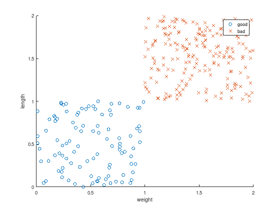
Plot the resulting data to discriminate.

axis equal
scatter(w(1:k),   l(1:k),   'o');  % good
hold on;
scatter(w(k+1:m), l(k+1:m), 'x');  % bad
xlabel('weight');
ylabel('length');
legend ({'good', 'bad'});

Classification

Looking at the figure above, it seems possible to find a seperating hyperplane. That is a linear function with unknown coefficients \(x_0\), \(x_1\), and \(x_2\)

\[\begin{split} f_{\text{linear}}(w_i,l_i) = x_0 + \begin{pmatrix} x_1 \\ x_2 \end{pmatrix}^{T} \begin{pmatrix} w_i \\ l_i \end{pmatrix} = x_0 + x_1 \cdot w_i + x_2 \cdot l_i \end{split}\]

to seperate

• the “good” blue cicles: \(f_{\text{linear}}(w_i,l_i) \leq -1\) for \(1 \leq i \leq k \leq m\) and

• the “bad” red crosses: \(f_{\text{linear}}(w_i,l_i) \geq 1\) for \(k < i \leq m\).

Note: \(w_i\) and \(l_i\) are the variables of \(f_{\text{linear}}(w_i,l_i)\)!

Feasibility problem as Linear Program (LP)

This classification problem can be formulated as LP:

\[\begin{split} \begin{array}{lrll} \textrm{minimize} & \begin{pmatrix} 0 & 0 & 0 \end{pmatrix} & x & \\ \textrm{subject to} & \begin{pmatrix} 1 & w_i & l_i \end{pmatrix} & x \leq -1, & i = 1, \ldots, k, \\ & -\begin{pmatrix} 1 & w_i & l_i \end{pmatrix} & x \leq -1, & i = k + 1, \ldots, m, \end{array} \end{split}\]

c = [0 0 0];
A = [ ones(k,  1),  w(1:k),    l(1:k); ...
     -ones(m-k,1), -w(k+1:m), -l(k+1:m) ];
b = -ones(m,1);
Aeq = []; % No equality constraints
beq = [];
lb = -inf(3,1);  % x0 to x2 are free variables
ub =  inf(3,1);
CTYPE = repmat ('U', m, 1);  % Octave: A(i,:)*x <= b(i)
x0 = [];  % default start value
%[x,~,exitflag] = linprog(c,A,b,Aeq,beq,lb,ub,x0);  % Matlab: exitflag=1 success
[x,~,exitflag] = glpk(c,A,b,lb,ub,CTYPE)            % Octave: exitflag=0 success

x =

  -23.712
   10.969
   11.999

exitflag = 0

The computed solution \(x\) are the sought coefficients for \(f_{\text{linear}}(w_i,l_i)\). Plotting the resulting function shows that it perfectly discriminates the measurements (test data).

axis equal
scatter(w(1:k),   l(1:k),   'o');  % good
hold on;
scatter(w(k+1:m), l(k+1:m), 'x');  % bad

f_quad = @(w,l) 1.*x(1) + w.*x(2) + l.*x(3);
ezplot (f_quad, [0,2,0,2]);

title ('');
xlabel('weight');
ylabel('length');
legend ({'good', 'bad', 'f_{linear}'});

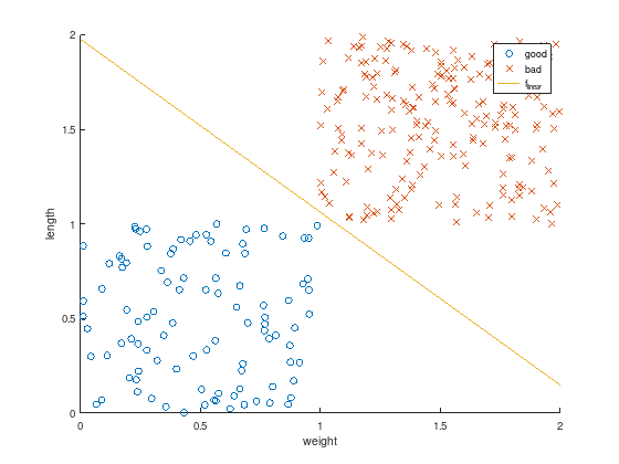
After this “training” the linear discrimination function \(f_{\text{linear}}(w_i,l_i)\) can be used to classify other data pairs as well.