MO01 - The illumination problem

Source: https://see.stanford.edu/Course/EE364A (hw3extra.pdf task 3).

A physical law from photometry states

\[ I = \frac{p}{r^{2}}\cos(\Theta), \]

the illuminance on a patch \(I\) (SI unit: lux \([lx = \frac{lm}{m^{2}}]\)) depends on:

1. the luminous intensity \(p\) (SI unit: candela \([cd = \frac{lm}{sr}]\)) of the lamps,

2. the distance to the respective patch \(r\) (SI unit: meter \([m]\)),

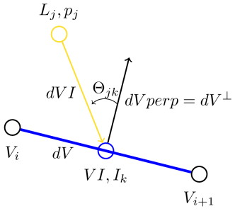
3. the angle \(\Theta\) to between the lamp and patch.

In case of the given problem data, there are \(m = 10\) lamps \(L_{j}\), \(j = 1, \ldots, m\), with assigned luminous intensities \(p_{j}\) and \(n = 20\) patches with respective illumination values \(I_{k}\), \(k = 1, \ldots, n\).

In the following the SI units are neglected. The following linear dependencies between \(I_{k}\) and \(p_{j}\) hold:

\[ I_{k} = \underbrace{\dfrac{1}{r_{kj}^{2}} \max(\cos(\Theta_{kj}), 0)}_{a_{kj}} \; p_{j} \]

with \(r_{kj} = \lVert dVI \rVert\) and

\[ \cos(\Theta_{kj}) = \dfrac{(dVI)^{T} (dVperp)}{\lVert dVI\rVert\cdot\lVert dVperp\rVert} \]

To regard all lamps \(p_{j}\), the luminous intensities have to be summed up:

\[ I_{k} = \sum_{j = 1}^{m} a_{kj} p_{j}. \]

Regarding all \(n = 20\) patches, the following overdetermined linear system of equation \(I = A \cdot p\) follows:

\[\begin{split} \begin{pmatrix} I_{1} \\ \\ \\ \vdots \\ \\ \\ I_{n} \end{pmatrix} = \begin{pmatrix} a_{1,1} & \cdots & a_{1,m} \\ \\ \\ \vdots & \ddots & \vdots \\ \\ \\ a_{n,1} & \cdots & a_{n,m} \end{pmatrix} \begin{pmatrix} p_{1} \\ \vdots \\ p_{m} \end{pmatrix}. \end{split}\]

As ultimate goal, all patch illuminations \(I_{k}\) should be as close as possible to the desired illumination \(I_{des}\).

Finally, the following constrained non-linear optimization problem can be formulated:

\[\begin{split} \begin{array}{ll} \textrm{minimize} & \displaystyle\max_{k = 1, \ldots, n} |\log{(I_{k})} - \log{(I_{des})}| \\ \textrm{subject to} & 0 \leq p_{j} \leq p_{max} \quad j = 1, \ldots, m. \end{array} \end{split}\]

The objective function formulates a quality measure \(f_{optimal}(p)\) depending on the luminous intensity of the lamps \(p_{j}\), that minimizes the maximal logarithmic distance between the actual patch illumination \(I_{k} = A_{(k,:)}p\) and the desired patch illumination \(I_{des}\).

\[\begin{split} \begin{aligned} f_{optimal}(p, I_{des}) :=& \max_{k = 1, \ldots, n} \lvert \log{(I_{k})} - \log{(I_{des})} \rvert \\ =& \max_{k = 1, \ldots, n} \lvert \log{(A_{(k,:)}p)} - \log{(I_{des})} \rvert \end{aligned} \end{split}\]

Last but not least, the constraints might seem trivial, but are for a practical application of importance: the luminous intensity of a lamp \(p_{j}\) has the physical constraints that it cannot “shine negative” and it cannot “shine brighter than possible”, \(0 \leq p_{j} \leq p_{\max}\).

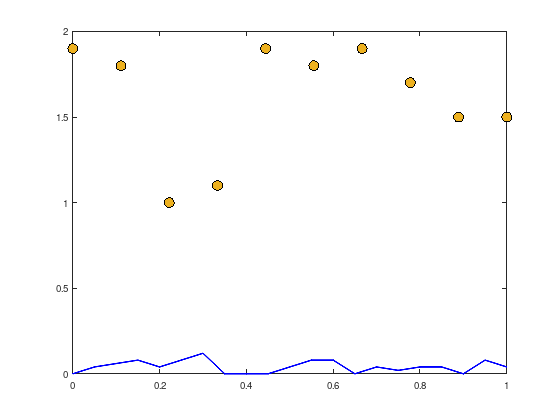
L = [linspace(0,1,10);
     1.9, 1.8, 1.0, 1.1, 1.9, 1.8, 1.9, 1.7, 1.5, 1.5];

m = size (L, 2); % number of lamps

% begin and endpoints of patches
V = [linspace(0,1,21);
     .4*[0.0, 0.1, 0.15, 0.2, 0.1, 0.2, 0.3, 0.0, 0.0, 0.0 , ...
         0.1, 0.2, 0.2, 0.0, 0.1, 0.05, 0.1, 0.1, 0.0, 0.2, 0.1]];
n = size (V, 2) - 1; % number of patches

plot (L(1,:), L(2,:), 'ko', 'MarkerSize', 10, ...
      'MarkerFaceColor', [0.9290 0.6940 0.1250]);
hold on;
plot (V(1,:), V(2,:), 'b-', 'LineWidth', 2);

% construct A
warning('off', 'Octave:colon-nonscalar-argument');
dV = V(:,2:n+1) - V(:,1:n); % tangent to patches
VI = V(:,1:n) +.5*dV;       % midpoint of patches
A = zeros (n, m);
for i = 1:n
  for j = 1:m
    dVI = L(:,j) - VI(:,i);
    dVperp = null (dV(:,i)'); % upward pointing normal
    if (dVperp(2) < 0)
      dVperp = -dVperp;
    end
    A(i,j) = max (0, dVI'*dVperp/...
      (norm(dVI)*norm(dVperp)))./norm(dVI)^2;
  end
end

Read task 3 from hw3extra.pdf and try to find an optimal solution with

1. Uniform \(p_{j}\)

2. Least-sqares

3. Linear Programming

4. Convex Programming (https://yalmip.github.io/ or http://cvxr.com/cvx/).

Solution hints.